【量化金融】量化指标的Python实现——Sharp比率、Sortino比率、Omega比率
|字数总计:1.6k|阅读时长:7分钟|阅读量:|
环境准备
测试用数据:demo_close_price_data点击下载
1
2
3
4
5
6
7
8
| import pandas as pd
import numpy as np
cp = pd.read_csv('close_price_demo.csv', encoding='gbk', index_col='date')
cp.index = pd.to_datetime(cp.index)
ret = cp.pct_change().iloc[1::]
cum_ret = (1+ret).cumprod()
cum_ret.plot(figsize=(10, 4))
|
1
2
3
4
5
6
7
8
9
10
11
12
13
14
15
16
17
18
19
20
21
22
23
24
25
|
BDAYS_PER_YEAR = 252
BDAYS_PER_QTRS = 63
BDAYS_PER_MONTH = 21
BDAYS_PER_WEEK = 5
DAYS_PER_YEAR = 365
DAYS_PER_QTRS = 90
DAYS_PER_MONTH = 30
DAYS_PER_WEEK = 7
MONTHS_PER_YEAR = 12
WEEKS_PER_YEAR = 52
QTRS_PER_YEAR = 4
def get_period_days(period):
period_days = {
'yearly': BDAYS_PER_YEAR, 'quarterly': BDAYS_PER_QTRS,
'monthly': BDAYS_PER_MONTH, 'weekly': BDAYS_PER_WEEK, 'daily': 1,
'monthly2yearly': MONTHS_PER_YEAR,
'quarterly2yearly': QTRS_PER_YEAR,
'weekly2yearly': WEEKS_PER_YEAR,
}
return period_days[period]
|
Sharp比率
Sharp比率(夏普比率)是衡量策略每承受一单位风险所产生的超额收益。夏普比率越高,表示单位风险下获得的超额收益越多。
其中涉及到了“无风险利率”的概念,大家应该知道,就是在进行毫无风险的投资的前提下,你能获得的最高收益率,一般使用国债收益率作为无风险利率。
获得回测期间投资策略的收益率rp,无风险收益rf,以及波动率σrp,便可以通过以下公式进行计算。
sharpe_ratio=σrpE(rp)−rf
应用时,我们一般使用年化的夏普比率,也就是把日频计算出的结果乘252
sharpe_ratio=σrp∗252(E(rp)−rf)∗252=σrp(E(rp)−rf)∗252
此处乘252的基本逻辑就如式中所示,分子乘252为年化收益,分母乘252为年化波动率;但是为何此处的年化收益不使用(1+r)252−1的方式进行计算?固然两者差异不大,尤其是在r比较小的时候,但是本质上还是有挺大差异。我也尝试使用比较成熟的金融计算库以及软件进行了测试,但大家都是默认了这样子的处理方式。
一直比较疑惑⊙﹏⊙∥
夏普比率大小参考:
| 阈值 | 等级 |
|---|
| sharp ratio<1 | 差 |
| 1<sharp ratio<1.99 | 中 |
| 2<sharp ratio<2.99 | 良 |
| 3<sharp ratio | 优 |
Python实现方式
1
2
3
4
5
6
7
8
| def sharpe_ratio(returns_df, risk_free=0, period='yearly'):
"""
计算(年化)夏普比率
"""
period_days = get_period_days(period)
sr = (returns_df.mean() - risk_free) * (period_days ** 0.5) / returns_df.std()
res_dict = {'sharpe_ratio': sr}
return res_dict
|
Sortino比率
Sortino比率与夏普比率类似,但只考虑下行风险,用于衡量策略在负波动市场中的绩效。
也就是我对亏损比赚钱更有兴趣,所以我把亏损的这部分拿出来算方差。因为很多时候正态分布是不对称的,我更看重亏钱部分会不会让我血本无归,赚钱部分也就是赚多赚少的区别。尤其是当Return的分布是左偏的时候,Sortino Ratio会比Sharpe Ratio更好用。
Sortinoratio=T1∑t=0T(Rpt−Rf)2E(Rp)−MAR (Rpt<MAR)
分子中,MAR就是Minimum Acceptable Return(可接受最低收益),在很多时候都等于无风险利率rf,但是不完全一致。
Python实现
1
2
3
4
5
6
7
8
9
10
11
| def sortino_ratio(returns_df, minimum_acceptable_return=0, period='yearly'):
"""
计算年化sortino比率
"""
period_days = get_period_days(period)
downside_returns = returns_df[returns_df < 0]
downside_volatility = np.std(downside_returns, axis=0)
excess_return = returns_df.mean() - minimum_acceptable_return
sr = excess_return*(period_days**0.5) / downside_volatility
res_dict = {'sortino_ratio': sr}
return res_dict
|
Omega比率
Omega比率基于策略超额收益率的分布特征, 通过设定一个阈值收益率来衡量策略在超过该阈值时的收益相对于未超过该阈值时的收益的比例。它可以帮助投资者了解投资策略或替代方法在多大程度上降低了尾部风险。设定我们用于区分上下行收益的阈值为r,那么:
omega=∫−∞rF(x)dx∫r∞(1−F(x))dx
其中F(x)是收益率的累积分布函数,其含义为如图的分布函数中,绿色的“上行收益区域”的面积除以红色的“下行收益区域”的面积。
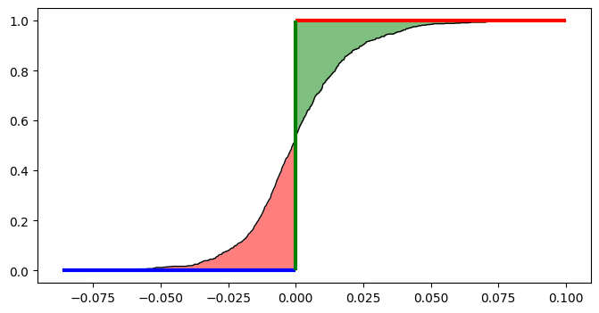
如果我们将图的分割粒度设置的粗一些,我们可以很简单的通过数学知识了解到,两个面积的比率事实上就是:
omega=−∑rp<rrp−r∑rp>rrp−r
Python实现
定义法
1
2
3
4
5
6
7
8
9
10
11
12
13
14
15
16
17
18
19
20
21
22
23
24
25
26
27
28
29
30
31
32
33
34
35
36
37
38
39
| def omega_ratio(returns_df, threshold=0, plot=False, bins=10000, period='daily'):
period_days = get_period_days(period)
threshold = (threshold + 1) ** (1 / period_days) - 1
hist, bin_edges = np.histogram(returns_df, bins=bins)
cdf = np.cumsum(hist/sum(hist))
result=list(zip(bin_edges[1::], cdf))
up_list=[i for i in result if i[0] > threshold]
down_list = [ i for i in result if i[0] < threshold]
up = 0
for i in range(len(up_list)-1):
x0 = up_list[i][0]
x1 = up_list[i + 1][0]
v = (x1 - x0) * (1 - up_list[i][1])
up += v
down=0
for i in range(len(down_list)-1):
x0 = down_list[i][0]
x1 = down_list[i + 1][0]
v = abs(x1 - x0) * (down_list[i][1])
down += v
omega = up / down
if plot:
fig, ax = plt.subplots(1, 1, figsize=(8, 4))
ax.plot(bin_edges[1::], cdf, linewidth=1, color='black')
ax.hlines(0, returns_df.min(), threshold, linewidth=3, colors='blue')
ax.hlines(1, returns_df.max(), threshold, linewidth=3, colors='red')
ax.vlines(threshold, 0, 1, linewidth=3, colors='green')
n = len(bin_edges[bin_edges<threshold])
ax.fill_between(bin_edges[1:n+1], cdf[0:n], 0, alpha=.5, linewidth=0, color='red')
ax.fill_between(bin_edges[n::], cdf[n-1::], 1, alpha=.5, linewidth=0, color='green')
res_dict = {'omega': omega}
return res_dict
|
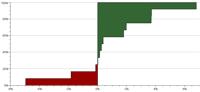
绘图部分比较粗糙,当bins比较小时,画的图会缺少一部分。
简单化简法
1
2
3
4
5
6
7
8
9
10
11
| def omega_ratio(returns_df, threshold=0, period='daily'):
"""
此处的period参数为说明输入的threshold为年化收益率还是日收益率
"""
period_days = get_period_days(period)
returns_less_thresh = returns_df - (1+threshold)**(1/period_days)+1
up = returns_less_thresh[returns_less_thresh > 0].sum()
down = -1 * returns_less_thresh[returns_less_thresh < 0].sum()
omega = up / down
res_dict = {'omega': omega}
return res_dict
|

 wechat
 alipay